Analog Proximity Sensors (0-10V/4-20mA): Linear Distance Measurement, Material Calibration, and PLC Scaling Guide
Standard discrete proximity switches operate on a binary logic state: ON or OFF. While effective for simple end-stop detection, binary switches cannot quantify how close an object is or track dynamic dimensional variations. When automated manufacturing requires continuous positioning, metal foil tension tracking, spindle eccentricity monitoring, or brake pad wear measurement, engineers specify analog proximity sensors.
Operating via high-frequency electromagnetic field damping, an analog inductive proximity sensor converts physical target displacement into a continuous, proportional electrical signal (0 to 10V DC, 0 to 20mA, or 4 to 20mA). This engineering manual details the operational physics of eddy current damping, evaluates voltage versus current signal architectures, provides material slope correction matrices, outlines complete Bedook Analog Series (M8, M12, M18, M30, and Q40) technical specifications, and provides executable PLC calibration routines for Siemens TIA Portal and IEC 61131-3 controllers.
1. Operational Physics: Electromagnetic Damping to Continuous Signal
Unlike digital inductive switches that feed an oscillator output into a Schmitt trigger comparator to generate a step-voltage pulse, an analog proximity sensor utilizes a linear demodulator circuit that directly samples oscillator amplitude decay.
- Resonant Field Generation: The sensor’s LC resonant circuit generates a high-frequency alternating electromagnetic field focused through a semi-shielded ferrite core at the sensing face.
- Eddy Current Loss: When a conductive metal target enters this electromagnetic field, circular eddy currents are induced on the metal surface according to Faraday’s law of induction.
- Impedance Damping: These eddy currents generate a counter-magnetic field (Lenz’s Law), drawing electrical energy away from the sensor’s LC tank. The closer the target approaches, the higher the energy absorption and the lower the oscillation amplitude.
- Linearized Output Conditioning: Instead of slicing this envelope at a single threshold, a precision internal analog conditioning circuit linearizes the non-linear oscillator envelope into a calibrated, proportional 0–10V or 0–20mA analog output.
2. Output Architecture: 0–10V Voltage vs. 0–20mA / 4–20mA Current Loops
Specifying the proper electrical output interface directly dictates measurement accuracy, cable run distances, and electromagnetic immunity across industrial control networks.
| Design Metric | Analog Voltage Output (0–10V DC) | Analog Current Output (0–20mA / 4–20mA) | Dual Output (Voltage + Current) |
|---|---|---|---|
| Bedook Model Code | Code “V” (e.g., CV2P2) | Code “I” (e.g., CI2P2) | Code “M” (e.g., CM2P2 / PM2S12) |
| Wiring Topology | 3-Wire (Brown: +V, Blue: 0V, Black: V_out) | 3-Wire (Brown: +V, Blue: 0V, Black: I_out) | 4-Wire (Black: V_out, White: I_out) |
| Permissible Load | High input impedance: > 2,000 Ω (≥ 4.7 kΩ) | Loop resistance: ≤ 400 Ω (≤ 0.4 kΩ) | V: ≥ 4.7 kΩ | I: ≤ 400 Ω concurrently |
| Cable Transmission Limit | ≤ 10 meters (susceptible to line drop) | ≤ 300 meters (impervious to wire resistance) | V local (≤ 5m) + I remote (≤ 200m) |
| EMI / Noise Immunity | Moderate. Induced VFD noise couples into ADC. | High. Closed current loop rejects common-mode noise. | High on Current output channel. |
| Wire Break Detection | Requires 1-10V scaling; 0V cannot distinguish cut wire. | 4-20mA allows automatic < 3.6mA wire-break trip. | Hardware redundancy across both channels. |
The Dual-Output (Code “M”) Advantage: Bedook M18, M30, and Q40 analog proximity sensors feature integrated dual simultaneous outputs. A control engineer can route the 0–10V output directly to a local operator console digital display, while routing the 0–20mA signal over a 150-meter cable tray to the centralized PLC cabinet without purchasing an external signal splitter.
3. Characteristic Transfer Curves: Blind Zone, Linear Range, and Saturation
Every inductive analog sensor exhibits a characteristic S-curve behavior. Precision automation requires configuring the machine stroke strictly within the Linear Measuring Range (sl):
- Blind Zone (Dead Zone, s < smin): Extremely close to the sensing face, the oscillator amplitude damping becomes non-linear. The output clamps near 0V or 0mA / 4mA. Do not use this zone for continuous positioning.
- Linear Operating Range (smin ≤ s ≤ smax): The calibrated working envelope where output current/voltage exhibits strict linear correlation (Linearity ≤ 5% of full scale, Repeatability < 2%).
- Saturation / Cutoff Zone (s > smax): Beyond the maximum rated distance, electromagnetic coupling dissipates. The output reaches maximum ceiling (10V or 20mA) and stays constant regardless of further target departure.
Bedook Analog Linear Range Matrix (Flush vs. Non-Flush)
| Form Factor | Mounting Execution | Linear Range (smin – smax) | Transfer Slope (Voltage: 0–10V) | Transfer Slope (Current: 0–20mA) | Frequency Response |
|---|---|---|---|---|---|
| M8 Threaded | Flush (BAB-M81.5) | 0.1 – 1.5 mm | 7.14 V / mm | 14.28 mA / mm | 100 Hz |
| Non-Flush (BAN-M82.5) | 0.1 – 2.5 mm | 4.16 V / mm | 8.33 mA / mm | 100 Hz | |
| M12 Threaded | Flush (BAB-M1203) | 0.1 – 3.0 mm | 3.45 V / mm | 6.90 mA / mm | 100 Hz |
| Non-Flush (BAN-M1204) | 0.1 – 4.0 mm | 2.56 V / mm | 5.12 mA / mm | 100 Hz | |
| M18 Threaded | Flush (BAB-M1804) | 1.0 – 4.0 mm | 3.33 V / mm | 6.67 mA / mm | 100 Hz |
| Non-Flush (BAN-M1807) | 1.0 – 7.0 mm | 1.66 V / mm | 3.33 mA / mm | 100 Hz | |
| M30 Threaded | Flush (BAB-M3010) | 5.0 – 10.0 mm | 2.00 V / mm | 4.00 mA / mm | 100 Hz |
| Non-Flush (BAN-M3014) | 7.0 – 14.0 mm | 1.43 V / mm | 2.86 mA / mm | 100 Hz | |
| Q40 Rectangular | Non-Flush (BAN-Q4025) | 5.0 – 25.0 mm | 0.50 V / mm | 1.00 mA / mm | 30 Hz |
4. Target Metal Reduction Factors & Output Slope Calibration
All catalog specifications are established using a grounded standard target: a flat sheet of Mild Carbon Steel (FE 360, 1mm thick). When monitoring non-ferrous metals, the material’s magnetic permeability and electrical conductivity alter the rate of eddy current generation, altering both the effective measuring range and the volts-per-millimeter transfer slope.
| Target Material | Correction Factor (Km) | Effective Range (Based on 1.0–7.0mm M18) | Slope Drift Impact |
|---|---|---|---|
| Mild Steel (FE 360) | 1.00 | 1.00 – 7.00 mm (100%) | Nominal slope (1.66 V/mm, 3.33 mA/mm) |
| Stainless Steel (AISI 304) | 0.75 – 0.80 | 1.00 – 5.60 mm (80%) | Slope steepens by ~25%; recalibrate PLC span. |
| Brass (CuZn) | 0.45 – 0.50 | 1.00 – 3.50 mm (50%) | Slope steepens by ~100%; reduced stroke. |
| Aluminum (Al) | 0.35 – 0.40 | 1.00 – 2.80 mm (40%) | Requires mounting sensor closer to aluminum target. |
| Copper (Cu) | 0.30 – 0.35 | 1.00 – 2.45 mm (35%) | Requires non-flush housing or M30 size to gain range. |
5. Bedook Analog Proximity Sensor Hardware Selection Matrix
The following engineering matrix details standard production part numbers across Bedook’s analog inductive product line:
| Model Number | Form Factor | Mounting | Linear Range | Output Signal | Supply Voltage | Termination | Housing Material |
|---|---|---|---|---|---|---|---|
| BAB-M81.5-CI2P2 | M8 × 1 | Flush | 0.1 – 1.5 mm | 0 – 20 mA | 18 – 30V DC | 2m PVC Cable | Nickel-Plated Brass |
| BAB-M81.5-CV2S8 | M8 × 1 | Flush | 0.1 – 1.5 mm | 0 – 10 V DC | 18 – 30V DC | M8 3-Pin Plug | Nickel-Plated Brass |
| BAN-M82.5-CV2P2 | M8 × 1 | Non-Flush | 0.1 – 2.5 mm | 0 – 10 V DC | 18 – 30V DC | 2m PVC Cable | Nickel-Plated Brass |
| BAB-M1203-CI2S12 | M12 × 1 | Flush | 0.1 – 3.0 mm | 0 – 20 mA | 18 – 30V DC | M12 4-Pin Plug | Nickel-Plated Brass |
| BAN-M1204-CV2S12 | M12 × 1 | Non-Flush | 0.1 – 4.0 mm | 0 – 10 V DC | 18 – 30V DC | M12 4-Pin Plug | Nickel-Plated Brass |
| BAB-M1804-CM2P2 | M18 × 1 | Flush | 1.0 – 4.0 mm | 0–20mA + 0–10V Dual | 18 – 30V DC | 2m PVC Cable (4-Wire) | Nickel-Plated Brass |
| BAN-M1807-CM2S12 | M18 × 1 | Non-Flush | 1.0 – 7.0 mm | 0–20mA + 0–10V Dual | 18 – 30V DC | M12 4-Pin Plug | Nickel-Plated Brass |
| BAB-M3010-CM2S12 | M30 × 1.5 | Flush | 5.0 – 10.0 mm | 0–20mA + 0–10V Dual | 18 – 30V DC | M12 4-Pin Plug | Nickel-Plated Brass |
| BAN-M3014-CM2P2 | M30 × 1.5 | Non-Flush | 7.0 – 14.0 mm | 0–20mA + 0–10V Dual | 18 – 30V DC | 2m PVC Cable (4-Wire) | Nickel-Plated Brass |
| BAN-Q4025-PM2S12-S | 40 × 40 × 54 mm | Non-Flush | 5.0 – 25.0 mm | 0–20mA + 0–10V Dual | 18 – 30V DC | M12 4-Pin Plug | Engineering PBT Block |
6. Electrical Wiring & Noise Suppression Best Practices
Industrial analog circuits are vulnerable to high-voltage electromagnetic interference (EMI) generated by variable frequency drives (VFDs) and servo motors. Follow these wiring schematics according to IEC 60947-5-2:
3-Wire Voltage (Code “V”) & Current (Code “I”) Pinout
- Pin 1 (Brown Wire): Connect to +24V DC (Permissible range: +18V to +30V DC).
- Pin 3 (Blue Wire): Connect to 0V DC Common Ground (GND).
- Pin 4 (Black Wire): Connect to PLC Analog Input Channel (+ Analog In).
4-Wire Dual Output (Code “M”) Pinout
- Pin 1 (Brown Wire): +24V DC Power
- Pin 3 (Blue Wire): 0V DC Common Ground
- Pin 4 (Black Wire): 0–10V DC Analog Voltage Signal Output
- Pin 2 (White Wire): 0–20mA Analog Current Signal Output
- Always use shielded twisted-pair cabling (e.g., Bedook PUR or PVC shielded accessory cables).
- Single-Ended Star Grounding: Connect the braided cable shield to functional earth (FE) ground only at the PLC control cabinet terminal strip. Never ground the shield at both ends; this creates circulating ground loops that inject 50/60Hz hum into the analog measurement.
- Route sensor analog cables in isolated raceways separated by at least 200mm from 3-phase AC motor leads and contactor coils.
7. PLC Mathematical Calibration & Scaling (TIA Portal S7-1200 / 1500)
Industrial PLC analog input modules (such as Siemens SM 1231 AI 4×13 Bit) digitize incoming 0–10V or 0–20mA signals into raw integer values ranging from 0 to 27648 (standard resolution).
The Universal Linear Scaling Equation
Distance (mm) = s_min + [ (Raw_Value − Raw_Min) / (Raw_Max − Raw_Min) ] × (s_max − s_min)
Executable Structured Text (ST / SCL) Code Block
Deploy this calibrated function block to convert raw analog words into calibrated physical millimeters, incorporating a first-order low-pass filter to dampen mechanical vibration:
FUNCTION_BLOCK "FB_Bedook_Analog_Scaling"
VAR_INPUT
    Raw_Input       : INT;     // Raw integer from %IW address (0 to 27648)
    s_min           : REAL;    // Minimum linear distance in mm (e.g., 1.0 for M18 Non-Flush)
    s_max           : REAL;    // Maximum linear distance in mm (e.g., 7.0 for M18 Non-Flush)
    Filter_Alpha    : REAL;    // Low-pass filter coefficient (0.0 to 1.0, typical: 0.15)
END_VAR

VAR_OUTPUT
    Distance_mm     : REAL;    // Scaled distance output in millimeters
    Sensor_Fault    : BOOL;    // Over-range or wire-break diagnostic flag
END_VAR

VAR
    Raw_Normalized  : REAL;
    Distance_Unfilt : REAL;
    Prev_Distance   : REAL;
END_VAR

BEGIN
    // 1. Boundary and Diagnostic Verification (Wire-Break / Short-Circuit)
    IF (Raw_Input < -200) OR (Raw_Input > 30000) THEN
        Sensor_Fault := TRUE;
        Distance_mm := 0.0;
        RETURN;
    ELSE
        Sensor_Fault := FALSE;
    END_IF;

    // 2. Normalization (0 to 27648 mapped to 0.0 to 1.0)
    Raw_Normalized := INT_TO_REAL(LIMIT(IN:=Raw_Input, MN:=0, MX:=27648)) / 27648.0;

    // 3. Physical Linear Scaling to Target Range
    Distance_Unfilt := s_min + (Raw_Normalized * (s_max - s_min));

    // 4. First-Order Digital Filter (Dampens Mechanical Chatter)
    Distance_mm := (Filter_Alpha * Distance_Unfilt) + ((1.0 - Filter_Alpha) * Prev_Distance);
    Prev_Distance := Distance_mm;
END_FUNCTION_BLOCK
8. High-Precision Industrial Application Scenarios
1. High-Speed Spindle Radial Runout & Shaft Eccentricity
On CNC machining centers and high-speed precision balancing rigs, bearing wear causes microscopic orbital precession. Positioning a Bedook BAB-M81.5-CV2S8 (Linear range: 0.1 to 1.5 mm, 100 Hz response) perpendicular to the polished shaft journal captures dynamic peak-to-peak voltage fluctuations, enabling automated preventative maintenance shutdowns before spindle seizure occurs.
2. Continuous Metal Sheet Thickness Verification
In automated stamping and roll-forming lines, dual coils or thickness deviations will destroy stamping dies. Mounting two calibrated BAB-M1203-CI2S12 sensors opposing a precision calibrated reference roller provides differential measurement down to ±15 μm resolution, reliably detecting doubled sheet metal feeds.
3. Dancer Arm Loop & Web Tension Control
In steel strip slitters and copper foil uncoilers, maintaining consistent tension requires monitoring the floating dancer roll height. Specifying the long-range BAN-Q4025-PM2S12-S (5.0 to 25.0 mm stroke) delivers continuous position feedback without mechanical potentiometers that wear out from continuous oscillation.
9. Frequently Asked Questions (FAQ)
What is the difference between an inductive proximity switch and an analog proximity sensor?
A standard proximity switch outputs a digital binary signal (ON or OFF) when a target crosses a fixed threshold distance. An analog proximity sensor continuously measures target distance across its working range, outputting a proportional 0–10V or 4–20mA signal that reflects exact position changes in real time.
Why does an analog sensor’s reading change when the target metal changes from steel to aluminum?
Inductive sensors operate via eddy currents. Aluminum has higher electrical conductivity and lower magnetic permeability than steel, creating lower impedance damping at equivalent distances. An aluminum plate yields a lower voltage/current output than mild steel at the same distance, requiring scaling recalibration in the PLC.
Should I choose 0–10V or 4–20mA for my control system?
Select 0–10V (Code “V”) if your sensor cable is short (≤ 5 meters) and terminates into a local panel meter or benchtop controller. Select 4–20mA or 0–20mA (Code “I”) if the cable runs long distances through factory trays adjacent to VFD motor cables; current signals are immune to wire resistance line-drop and electromagnetic noise.
Can I mount two analog proximity sensors side-by-side?
Mounting analog sensors too close together causes mutual electromagnetic crosstalk, appearing as cyclic signal oscillation in the PLC. Maintain a minimum center-to-center spacing of at least ≥ 3 × Sensor Diameter for flush models, and ≥ 6 × Sensor Diameter for non-flush models.
Source Factory-Direct Analog Sensing Hardware
Achieve sub-millimeter displacement feedback without investing in fragile laser optical systems or expensive linear encoders. Bedook manufactures a complete catalog of industrial analog inductive proximity sensors.
- Control Systems Engineers: Download complete electrical schematics, 2D dimensional prints, and 3D STEP CAD models for M8, M12, M18, M30, and Q40 analog series.
- OEM Procurement Specialists: Contact our technical sales desk for volume-tiered factory-direct pricing, application compatibility testing, and rapid sample fulfillment within 24 hours.
Explore Bedook: Your Trusted Sensor Manufacturer
At Bedook, we specialize in designing, developing, and manufacturing a comprehensive range of proximity sensors and switches. Our extensive product lineup includes:
- Inductive Proximity Sensors
- Capacitive Proximity Sensors
- Photoelectric Sensors
- Ultrasonic Sensors
- Solid State Relays
- Various Accessories
With over 10,000 detailed product variations and a robust R&D team, we take pride in our ability to meet your unique requirements with tailored solutions and reliable performance.
Whether you’re seeking off-the-shelf products or customized designs, Bedook offers the expertise and production capacity to ensure your satisfaction.
Get in Touch Today!
We value your interest in our products and warmly encourage you to send us an inquiry. Let us help you find the perfect sensor solution for your application.
Thank you for considering Bedook—your trusted partner in innovation and quality manufacturing. We look forward to collaborating with you!
 Capacitive Proximity Sensor Selection Guide: Dielectric Constants, Liquid Level, and Non-Metallic Target Detection